The Gloucester subregion is defined by the geological Gloucester Basin (Roberts et al., 1991). As this is a geological mapping unit, there has been no consideration beyond the subregion boundary of groundwater and/or surface water connection.
Over the last ten years the regional hydrogeology of the Gloucester subregion has been characterised during commercial assessment of energy resources (there are no other sources) and no groundwater connectivity has been found beyond the Gloucester subregion (Parsons Brinckerhoff, 2012a, pp. xxv, 30, 31; SRK, 2010, p. 45). From a groundwater perspective it is a closed system with groundwater discharging to lower portions of the landscape and being evaporated through riparian vegetation (Parsons Brinckerhoff, 2012a, pp. 30‑31). Hence, as there is no groundwater connection to assets beyond the boundary of the Gloucester subregion, no further consideration of groundwater connectivity is required.
By contrast, there are surface water connections beyond the boundary of the Gloucester subregion that need to be considered. The Gloucester subregion straddles the headwater of two surface water basins (Figure 3) and covers about 347.5 km2 – of this, the north‑flowing component (see ‘N’ in Figure 3) is 181.2 km2 and 166.3 km2 comprises the south‑flowing component (see ‘S’ in Figure 3).
The Australian Hydrological Geospatial Fabric (Geofabric) – developed by the Bureau of Meteorology (2012) – was used to define a set of catchments that flow into and out of the northern and southern components of the Gloucester subregion (Figure 3). This process identified 13 subcatchments (Figure 3). Seven subcatchments define the north flowing rivers that comprise the Manning river basin, five subcatchments constitute the south flowing rivers that make‑up the Karuah river basin, the remainder is the Wallamba River catchment. As the Wallamba River catchment (in which the town of Forster is located; see Figure 3) is not hydrologically connected to surface water flowing from the Gloucester subregion, it is not considered further. The names, areas and codes of the 13 subcatchments used herein are provided in Table 4.

Figure 3 Location of the Gloucester subregion, within the Manning river basin and Karuah river basin
Some rivers from the Gloucester subregion flow north (denoted by the hot pink ‘N’ internal to the subregion boundary) into the Manning river basin, while others flow south (denoted by the hot pink ‘S’ internal to the subregion boundary) into the Karuah river basin. The codes for the subcatchments (developed and used here) are provided in brackets following the subcatchment name. Source data: The catchment boundaries and both the major and minor watercourses are from Geoscience Australia (2006).
Table 4 Details of subcatchments comprising the Manning and Karuah river basins and Wallamba river catchment as identified in Figure 3
The PAE is the geographic area associated with a bioregion or subregion in which the potential water‑related impact of coal resource development on assets is assessed. It is the first step to identify the potentially impacted assets. Given that the Gloucester subregion is only connected externally via surface water, there is a need to know the relative proportions flowing from the subregion compared to those generated from other parts of the Manning and Karuah river basins – for example, in the Manning river basin to answer the question ‘what proportion of the streamflow at Taree is generated from runoff originating in the northern flowing component of the Gloucester subregion?’ As there is only limited streamflow gauging on the surface water network in the broader region within which the Gloucester subregion is located, there is insufficient observational data available to answer this question. Thus spatially explicit surface water modelling was undertaken; this modelling is documented in the remainder of this subsection.
Over the long‑term, the relative proportion of the streamflow generated in a catchment relates to its area and more importantly to the spatial change in climate across the catchment (Budyko, 1974; Donohue et al., 2011). For a general introduction to the Budyko framework see Donohue et al., (2007; 2010); the following brief introduction is from McVicar et al. (2012). The Budyko framework is widely used; according to Google Scholar (a freely accessible web search engine that indexes the full text of scholarly literature across an array of publishing formats and disciplines; Google Scholar, 2014) using the search ‘Budyko M.I. Climate and Life’ shows that it has been cited in the international scientific literature over 1600 times. The Budyko framework addresses water quantity issues, and water quality, as represented by in‑stream electrically conductivity, can be regarded as high quality throughout the subregion. So water quality issues are not considered when defining the PAE.
The catchment water balance describes the partitioning of the inward flux, or supply, of water (assumed here to be solely precipitation) into the outward fluxes of water and the within‑catchment storage of water. With respect to streamflow, the water balance is:
|
|
(1) |
here Q, P, AET, and DD represent streamflow, precipitation, actual evapotranspiration and deep drainage, respectively (mm a‑1). Sw is soil water storage (mm). In unregulated catchments the partitioning of P into Q and AET predominantly depends on the processes that determine AET. In general, AET is limited by either the supply of: (i) water or (ii) energy (this can be termed atmospheric evaporative demand (AED) and is commonly represented as potential evapotranspiration (PET). This means that AET from a catchment can be described as being either ‘water‑limited’ or ‘energy‑limited’, respectively. This supply‑demand limitation is a crucial over‑arching framework for understanding catchment hydroclimatology; it does not account for changes in soil properties and assumes groundwater and surface water are in steady‑state equilibrium with groundwater recharge and discharge being negligible.
Assuming steady state, Budyko (1974) described long‑term catchment balances using the supply‑demand framework (Figure 4). Formally, a water‑limited environment occurs when the long‑term catchment average AED for water exceeds the supply of water (i.e. P < PET) and the opposite is true for an energy‑limited environment (i.e. P > PET). Over large catchments and long time‑scales, Budyko showed that the evaporative index (e, the ratio of AET to P) is dependent on the climatic dryness index (F, the ratio of PET to P) and closely follows a curvilinear relationship (the ‘Budyko curve’, shown in Figure 4). As water limitation increases (i.e. as one moves to the right in Figure 4), then AET approaches P and Q approaches 0. Conversely, as the water availability increases (i.e. as one moves to the left in Figure 4), AET approaches PET, with a larger fraction of P being partitioned into Q.

Figure 4 The Budyko curve and the supply-demand framework
The Budyko curve (black line) describes the relation between the long‑term catchment averages of the evaporative index (e = AET / P) and the dryness index (F = PET / P). The horizontal grey line represents the water‑limit, where 100% of P becomes AET, and the diagonal grey line is the energy‑limit, where 100% of AED (i.e., PET) is converted to AET. The green shaded area represents the fraction of P that becomes AET and the blue shaded area represents the fraction of P that becomes Q.
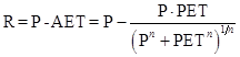
Using Choudhury’s (1999) formulation of the Budyko curve, with (i) available energy being more commonly represented as PET (Donohue et al., 2012, whereas Choudhury originally used net radiation), (ii) n being the catchment properties parameter that alters the partitioning of P between modelled AET and R (runoff) and using a value of 1.9 here (Donohue et al., 2011) and (iii) assuming steady state conditions, then R is simply the difference between P and AET:
|
|
(2) |
Using readily available gridded meteorological datasets of P (Jones et al., 2009) and Penman’s formulation of PET (Donohue et al., 2010), which is fully physically based using a dynamic wind speed (McVicar et al., 2008), Choudhury’s formulation of the Budyko framework was used to model the climatological (1982 to 2010) partitioning of P in AET and R. Figure 5a and Figure 5b show the input meteorological grids used in Choudhury’s formulation of the Budyko framework; the resultant modelled runoff is shown in Figure 5c. Note that in the introduction to the Budyko framework, in which the smallest spatial element considered is a subcatchment, Q is used, whereas for spatially explicit modelling using gridded meteorological data the term R is used. These are not identical in meaning and in the Budyko framework there is no routing within a catchment or down the river network. To define the PAE it is only the spatially explicit relative proportions of R that are required.

Parts (a) and (b) show annual average (1982 to 2012) precipitation and potential evapotranspiration, respectively. These are input to Choudhury’s formulation of the Budyko framework to provide the modelled annual average (1982 to 2012) runoff which is shown in (c).
The input P and PET grids and the resultant R grid were then summarised by the 13 subcatchments (Figure 3 and Table 4), and were then expressed as a percentage of the totals determined for each of the Manning and Karuah river basins; see Table 5. This shows that the northern component of the Gloucester subregion (see Figure 3) contributes 2.16, 2.16 and 2.11 % of P, PET and R, respectively, to the Manning river basin totals of these long‑term water balance components. The southern component of the Gloucester subregion (see Figure 3) contributes 5.22, 5.68 and 4.64% of P, PET and R, respectively, to the Karuah river basin totals of these long‑term water balance components (Table 5).
Table 5 Annual average water balance components for the Manning and Karuah river basins
The annual average (1982 to 2010) water balance components are shown for precipitation, potential evapotranspiration (PET calculated with the Penman formulation) and Choudhury’s modelled runoff for each of the subcatchments. Percentages are calculated relative to the respective river basin totals. Definitions for the subcatchment codes are provided in Table 4, and their locations are illustrated in Figure 3.
By considering the surface water subcatchment topology (i.e. their spatial relationships of inflow, outflow and tributaries) it is possible to accumulate the percentage contributions of the northern component of the Gloucester subregion (see Figure 3) down the Manning River to its outflow in the Tasman Sea (Table 6). In the following text, only results for R are discussed; the values for P and PET are provided for completeness in Table 6. Table 6 shows that the northern component of the Gloucester subregion contributes 57.18% of the R of N2 and, when considering the inflow from N1 to N2, this decreases to 28.40%. When considering the inclusive streamflow from N1 to N4, the contribution of the northern component of the Gloucester subregion reduces to 9.57%, and when the additional contribution of N5 is considered then the northern component of the Gloucester subregion only contributes 3.01% of the runoff from the area composed of N1, N2, N3, N4 and N5 (see Table 6 and, for locations, Figure 3). Based on expert opinion, at approximately 10% of the runoff there may be the ability to detect the impact of changes in runoff, but at less than 5% of the total runoff, even if the change did have an impact, this is considered to be smaller than the detection level. This suggests that any change to surface water flows beyond the confluence of N4 and N5 is small and hence defines the northern component of the Gloucester PAE to include the major river channel flowing in N4, as in N6 and N7 there will be negligible influence of changes in surface water generated from N due to the relatively large contribution from N5 (i.e. 48.11% from Table 5) to the entire Manning river basin.
Table 6 Accumulated percent contribution of water balance components from the northern component of the Gloucester subregion relative to selected parts of the Manning river basin
The annual average (1982 to 2012) water balance components are shown for precipitation, potential evapotranspiration (PET calculated with the Penman formulation) and Choudhury’s modelled runoff. The percentage contributions of the northern component relative to the subcatchments, indicated by the denominator, are reported. Definitions for the subcatchment codes are provided in Table 4, and their locations are illustrated in Figure 3.
The southern component of the Gloucester subregion (see Figure 3) in the Karuah river basin was assessed in a similar manner to that used for the accumulated percentage contributions of the northern component of the Gloucester subregion. Table 7 shows that the southern component of the Gloucester subregion contributes 47.43% of the R of S2 and, when considering the inflow from S1 to S2, this decreases to 22.23%. When inflow from S3 is considered the contribution of the southern component of the Gloucester subregion reduces to 10.19% when the Karuah River flows into the western end of Port Stephens. When considering surface water flow into all of Port Stephens (i.e. S1+S2+S3+S4+S5, see Figure 3) the contribution of the southern component of the Gloucester subregion reduces to 4.64%. This suggests that any change to surface water flows to all of Port Stephens due to changes in the southern component of the Gloucester subregion will be negligible. This then means that not all of Port Stephens is considered in the PAE. The extension to the PAE of the Gloucester subregion is defined as the reach of the Karuah River that flows south from the southern component of the Gloucester subregion to the western end of Port Stephens (Figure 6).
Table 7 Accumulated percent contribution of water balance components from the southern component of the Gloucester subregion to selected parts of the Karuah river basin
The annual average (1982 to 2012) water balance components are shown for precipitation, potential evapotranspiration (PET calculated with the Penman formulation) and Choudhury’s modelled runoff. The percentage contributions of the southern component relative to the subcatchments, indicated by the denominator, are reported. Definitions for the subcatchment codes are provided in Table 4, and their locations are illustrated in Figure 3.
The PAE of the Gloucester subregion is comprised of the union of the Gloucester subregion boundary and, to account for changes in surface water flows, 1 km buffer zones either side of the major rivers flowing from the northern component (to the outlet of N4) and from the southern component to Port Stephens (Figure 6). The Australian Bureau of Statistics (ABS, 2012, Table 4) reported an estimate of the total area of farm holdings and number of agricultural businesses for each local government area (LGA) as at 30 June 2011. For the Gloucester LGA the area is 129,354 ha held by 323 businesses, having an average size of approximately 400 ha. For Great Lakes LGA there is 67,885 ha held by 305 businesses, with an average area of approximately 222 ha. The average of these two areas (311 ha or 3.1 km2) is, relative to all NSW (ABS, 2012), a small holding (due to the high rainfall and relative high population density of the subregion for a non‑urban area), and it is assumed that water from rivers will be pumped a maximum of 1 km.
The Gloucester subregion covers about 347.5 km2, with the area of the PAE being approximately 468.2 km2. This means that accounting for possible surface water connections beyond the subregion requires the PAE to be 120.7 km2 larger than the Gloucester subregion. It is in the PAE that geospatial referenced lists of water‑dependent assets will be identified.

Figure 6 Location of the Gloucester preliminary assessment extent (PAE)
The PAE comprises the subregion and a 1 km buffer either side of the north‑flowing Gloucester River until it joins the Manning River; a similar buffer is used for the south‑flowing Karuah River until it reaches Port Stephens.
