The purpose of a statistical emulator is to provide a computationally efficient surrogate for a computationally expensive model. These emulators provide a way to quantify the predictive distribution for a prediction of interest, given a new set of parameters for which the model was not run. Thus regional-scale model estimates can be updated at a site with information that better reflects local-scale conceptual models of the geology and hydrogeology. The predictions of interest are the groundwater hydrological response variables, dmax and tmax. Changes in the surface water – groundwater flux are incorporated into the streamflow modelling as changes in baseflow and inform the surface water hydrological response variables, reported in companion product 2.6.1 for the Hunter subregion (Zhang et al., 2018).
As outlined in the uncertainty analysis workflow (Figure 5 in Section 2.6.2.1), an emulator is created for each objective function (see Section 2.6.2.8.1) and for each prediction of drawdown due to additional coal resource development and year of maximum change. The objective function emulators are used in the Markov chain Monte Carlo sampling of the prior parameter distribution to create a posterior parameter distribution for each prediction. These posterior parameter distributions are subsequently sampled with the emulator for that prediction to produce the predictive distribution of drawdown and year of maximum change due to additional coal resource development at each model node.
The statistical emulation approach employed herein is called Local Approximate Gaussian Processes (LAGPs) as implemented through the ‘aGP’ function of the ‘laGP’ package (Gramacy, 2014) for R (R Core Team, 2013). LAGPs were chosen because: (i) they can be built and run very rapidly in the ‘laGP’ R package; (ii) unlike some other popular emulation approaches (e.g. standard Gaussian process emulators), they allow for nonstationarity in the model output across the parameter space, which provides the emulator with more flexibility to match model output; and (iii) they were found to have excellent performance when compared to a range of other emulation techniques (Nguyen-Tuong et al., 2009; Gramacy, 2014).
The training and evaluating of an individual emulator is implemented through a set of custom-made R-scripts with the following input requirements:
- design of experiment parameter combinations
- design of experiment model output
- transform of parameters
- transform of output.
The set of 1500 parameter combinations that were evaluated and their corresponding model results are used to train the individual emulators for each prediction.
Before training the emulator, the quantity to be emulated is transformed using a normal quantile transform (Bogner et al., 2012). The following steps are required to carry out such a normal quantile transformation of a sample X:
- Sort the sample X from smallest to largest:
 .
. - Estimate the cumulative probabilities
 using a plotting position like
  such that
 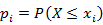 .
. - Transform each value
 of X in
  of the normal variate Y, where Q-1 is the inverse of the standard normal distribution, using a discrete mapping.
The main advantage of this transformation is that it transforms any arbitrary distribution of values into a normal distribution. Gaussian process emulators tend to perform better if the quantity to emulate is close to the normal distribution. The drawback of the transformation is that it cannot be reliably used to extrapolate beyond the extremes of the distribution. This risk is minimised in this application by purposely choosing the parameter ranges in the design of experiment to be very wide as to encompass the plausible parameter range. In a final step, the resulting value of the emulator is back-transformed to the original distribution.
The predictive capability of LAGP emulators is assessed via 30-fold cross validation (i.e. leaving out 1/30th of the model runs, over 30 tests) and recording diagnostic plots of the emulator’s predictive capacity. For each of the 30 runs of the cross-validation procedure, the proportion of 95% predictive distributions that contained the actual values output by the model (also called the hit rate) was recorded. The emulators are considered sufficiently accurate if the 95% hit rate is between 90 and 100%.
The accuracy of the emulator, the degree to which the emulator can reproduce the relationship between the parameters and the prediction, depends greatly on the density of sampling of parameter space. This section examines whether the set of 1500 evaluated parameter combinations provides sufficient information to train ten-dimensional emulators. As it is beyond the scope of this product to examine this for all the emulators created, the suitability of the number of parameter combinations is illustrated using the fraction of gauges for which the average historical baseflow is between the negative 20th percentile and the 70th percentile of observed total streamflow. Emulating this quantity is especially challenging as this fraction is a non-linear function of several interacting parameters.
Figure 32 shows the correspondence between the modelled and emulated fraction of the baseflow objective function (see Section 2.6.2.8.1) using an emulator trained with 100, 500, 1000 and 1500 samples. The performance is poor for emulators trained with 100, 500 and 1000 samples; however, the performance is adequate for the emulator trained with 1500 samples.
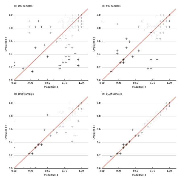
Data: Bioregional Assessment Programme (Dataset 2)
Figure 33 shows this evolution in a more quantitative way by visualising the mean absolute error between modelled and emulated values produced by emulators trained with training sets that vary from 100 to 1500 in increments of 100. This fraction is used as an objective function in the uncertainty analysis (see Section 2.6.2.8.1) in which parameter combinations are accepted if the fraction is in excess of 0.9. The mean absolute error of an emulator trained with 1500 samples is 1%. By using an emulator with this accuracy in the Markov chain Monte Carlo sampling, the risk of wrongly accepting or rejecting a parameter combination is very small. Emulators with this level of accuracy also provide confidence that predictions obtained with the emulators are very close to predictions generated with the original model.
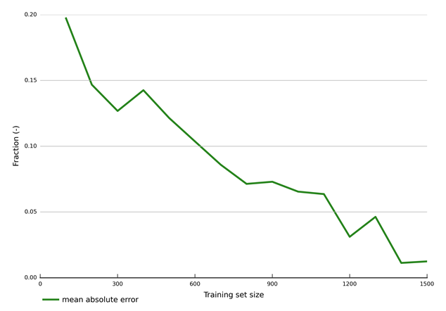
Data: Bioregional Assessment Programme (Dataset 2)
