8.1 Outputs for product 2.6.1 (surface water numerical modelling)
8.1.1 Hydrological response variables
8.1.1.1 Routine set of nine hydrological response variables
Product 2.6.1 (surface water numerical modelling) reports the potential impacts of coal resource development on water resources at the selected model nodes within the surface water modelling domain. This is done by comparing model simulations of the CRDP with those of the baseline. See Appendix B for recommended content to be included in product 2.6.1 (surface water numerical modelling).
Nine hydrological response variables have been chosen by BA ecological experts to characterise the impacts of coal resource development. These variables are intended to be representative of the flow characteristics that are important for assessing impacts on economic and ecological assets. To a large extent they are selected from the list of ecologically relevant streamflow metrics presented by Kennard et al. (2010). Five of the hydrological response variables characterise low streamflow, two characterise high streamflow, and two characterise long-term flow variability.
The low-streamflow hydrological response variables are:
- P01: the daily streamflow rate at the 1st percentile (ML/day)
- ZFD: the number of zero-flow days per year. Zero flow is identified using the minimum detectable flow. For ease of applicability, a threshold of 0.01 ML/day is set for determining the number of zero-flow days for all surface water nodes
- LFD: the number of low-flow days per year. The threshold for low-flow days is the 10th percentile from the simulated 90-year period (2013 to 2102)
- LFS: the number of low-flow spells per year (perennial streams only). A spell is defined as a period of contiguous days of streamflow below the 10th percentile threshold
- LLFS: the length (days) of the longest low-flow spell each year.
The high-streamflow hydrological response variables are:
- P99: the daily streamflow rate at the 99th percentile (ML/day)
- FD: flood (high-flow) days, the number of days with streamflow greater than the 90th percentile from the simulated 90-year period (2013 to 2102).
In addition, two hydrological response variables that represent streamflow volume and variability are:
- AF: the annual flow volume (GL/year)
- IQR: the interquartile range in daily streamflow (ML/day); that is, the difference between the daily streamflow rate at the 75th percentile and at the 25th percentile.
For each of these hydrological response variables a time series of annual values is constructed.
Some of these hydrological response variables are mutually exclusive. For example, a location with many zero-flow days is likely to have a P01 value of 0 ML/day. In general for a particular location, one or the other of these metrics is likely to produce useful information, but not both.
While the selection of these hydrological response variables for characterising important surface water impacts considers economic and ecological assets and spans the potential hydrological changes, the expert input into the receptor impact modelling (through qualitative models of potentially impacted landscape classes) might identify the system’s dependency on other key hydrological response variables which will be considered at that time. The priority in product 2.6.1 (surface water numerical modelling) is to routinely estimate a set of hydrological response variables that summarise the potential hydrological changes.
8.1.1.2 Additional hydrological response variables for receptor impact modelling
Any extra hydrological response variables identified through further expert input will not be described in product 2.6.1 (surface water numerical modelling) but will be carried forward to the analysis reported in product 2.7 (receptor impact modelling). In general, different additional hydrological response variables might be selected in different subregions. These additional hydrological response variables are likely to be presented as 30-year averages of occurrence frequencies. Examples of additional hydrological response variables might include:
- R0.3: the peak daily flow in flood events with a return period of 0.3 years is defined from modelled baseline flow in the reference period (1983 to 2012). In the future 30-year periods, we report the mean annual number of events with a peak daily streamflow exceeding this reference R0.3 value. This metric is designed to be approximately representative of over-bench flow events.
- R3.0: the peak daily flow in flood events with a return period of 3 years is defined from modelled baseline flow in the reference period (1983 to 2012). In the future 30-year periods, we report the mean annual number of events with a peak daily streamflow exceeding this reference R3.0 value. This metric is designed to be approximately representative of over-bank flow events.
- Qzero: the mean number of days per year with zero streamflow during a 30-year period. For practical and numerical reasons, zero streamflow is defined as any modelled streamflow below 10 ML/day. Note that its flow threshold is much higher than that used for the zero streamflow metric (ZFD) described in Section 8.1.1 . This Qzero metric is designed to be approximately representative of the flow rate at which all river pools will join up and form a continuously flowing reach.
Justification for these and any other additional metrics will be provided in product 2.7 (receptor impact modelling).
8.1.2 Criteria for analysing the impacts on hydrological response variables
Three criteria are selected to evaluate the change in each hydrological response variable. These three criteria are calculated for each of the 10,000 model run replicates of the uncertainty analysis. Each criterion is obtained from the annual time series of the relevant hydrological response variable.
The first criterion is the maximum absolute change in the hydrological response variable and is defined as:
|
|
(5) |
where A is the variable (hydrological response variable), t represents the tth prediction year, and the subscripts c and b represent the CRDP and the baseline, respectively.
Equation (5) describes the case where the additional coal resource development is expected to lead to increases in the value of A (e.g. the number of low flow days). In cases where the additional coal resource development is expected to lead to decreases in the value of A (e.g. the annual flow volume), the criterion ΔAmax is negative and is given by:
|
|
(6) |
The second criterion is the maximum percentage change in hydrological response variable and is defined as:
|
|
(7) |
where tmax is the year of maximum difference between Ac and Ab. This criterion is applicable for volumetric hydrological response variables (e.g. P01, P99, annual streamflow and interquartile range), but will not always be applicable for the other five hydrological response variables with days as units. This is because the five hydrological response variables under the baseline are likely to be equal to zero for many hydrological nodes (see Section 2.6.1.4.3) which makes Equation (7) invalid.
The third criterion is tmax, the year of maximum change (the year when ΔAmax is observed).
Each of these criteria will be reported in product 2.6.1 (surface water numerical modelling) for each model node. They will be presented in the form of boxplots representing the range of responses from the 10,000 model replicates. The output will follow this format regardless of whether it is derived from AWRA-L or a combination of AWRA-L and AWRA-R.
Figure 10 and Figure 11 provide examples of these boxplots for two hydrological response variables for 30 surface hydrological model nodes in the Gloucester subregion. In these figures ΔAmax is denoted as amax, ΔApc is denoted as pmax and tmax is denoted as tmax.

Figure 10 Example boxplot: the impact of additional coal resource development on streamflow at the 1st percentile (P01) at the 30 model nodes within the Gloucester subregion
Example only; do not use for analysis. This is an early draft of a figure published in Zhang et al. (2016). See Zhang et al. (2016) for full explanation and interpretation of the final results, which might vary from that shown here.
Numbers above the top panel are the median of the 10,000 replicates under the baseline for the year corresponding to the median tmax. In each boxplot, the bottom, middle and top of the box are the 25th, 50th and 75th percentiles, and the bottom and top whiskers are the 5th and 95th percentiles. The thick black line divides northern model nodes (1–17) and southern model nodes (18–30). The amax, pmax and tmax refer to the maximum absolute impacts, maximum percentage impacts and year of maximum change, respectively.
Receptor ID = model node ID
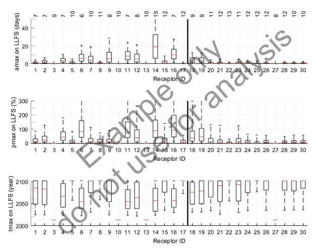
Figure 11 Example boxplot: the impact of additional coal resource development on the length of longest low-flow spell (LLFS) at the 30 model nodes within the Gloucester subregion
Example only; do not use for analysis. This is an early draft of a figure published in Zhang et al. (2016). See Zhang et al. (2016) for full explanation and interpretation of the final results, which might vary from that shown here.
Numbers above the top panel are the median of the 10,000 replicates under the baseline for the year corresponding to the median tmax. In each boxplot, the bottom, middle and top of the box are the 25th, 50th and 75th percentiles, and the bottom and top whiskers are the 5th and 95th percentiles. The thick black line divides northern model nodes (1–17) and southern model nodes (18–30). The amax, pmax and tmax refer to the maximum absolute impacts, maximum percentage impacts and year of maximum change, respectively.
8.1.3 Interpolation of hydrological changes
The predictions of streamflow from the landscape and river models are for specific locations in the stream network. These are termed the model nodes. It is at these model nodes that the hydrological response variables are derived.
For some applications in BA, particularly in relation to the river impact modelling, it may become necessary to provide hydrological response variable predictions for locations on the stream network that are not at model nodes. In other words, some degree of spatial interpolation or extrapolation will be required. Such an interpolation or extrapolation will allow entire stretches of particular riverine landscape classes to be associated with one or more streamflow regimes.
The simplest interpolation strategy is to simply adopt the flow volume (and associated hydrological response variables) from a nearby model node on the same streamline. Since model nodes are typically placed immediately upstream of major confluences, it is not unreasonable to expect that flow predictions at such a node will be representative of the flow for some distance along the reach upstream of the node. The distance along the reach over which this translation of flow prediction would be safe is dictated by the topology of the network and by proximity to additional coal resource development.
In some instances it may be appropriate to interpolate along part, but not all, of a reach. For example, it may be appropriate to interpolate upstream from a model node as far as the next significant inflow point. Alternatively, it may be appropriate to interpolate upstream from a node as far as an inflow point associated with a mining development.
This direct interpolation scheme may be inappropriate in some circumstances. In such cases, consideration could be given to implementing alternative interpolation strategies such as areal weighting of streamflows.
8.1.4 Zone of potential hydrological change
Product 2.6.1 (surface water numerical modelling) reports on the maximum differences between CRDP and baseline projections of the annual time series of nine hydrological response variables. Each of these variables are produced at every model node. Using the interpolation schemes outlined in Section 8.1.3, these projections can give estimates of the maximum hydrological change at any point along a reach.
It is important to recognise that the predicted hydrological changes represent the largest annual departure between the baseline and CRDP predictions for the respective hydrological response variables. As such, they represent extreme responses. They do not necessarily represent the magnitudes of responses that would be expected to occur every year.
However, they do provide a convenient means of discriminating between parts of the landscape that are potentially affected by additional coal resource development and those parts of the landscape that are almost certainly unaffected and can be ruled out from further analysis. The river reaches that are potentially affected – that is, those reaches where changes in one or more hydrological response variables exceed the specified thresholds – are within the zone of potential hydrological change (which includes the extent of potential changes in both surface water and groundwater).
For the flux-based hydrological response variables (AF, P99, IQR and P01), the threshold for inclusion in the surface water zone of potential hydrological change is a greater than 5% chance of there being at least a 1% change in the variable. That is, if 5% or more of model replicates show a maximum difference between CRDP and baseline projections of 1% or more (relative to the baseline value). For four of the frequency-based metrics (FD, LFD, LLFS and ZFD), the threshold is a greater than 5% chance of there being a change in the variable of at least 3 days in any year. For the final frequency-based metric (LFS), the threshold is a greater than 5% chance of there being a change in the variable of at least 2 spells in any year.
A node and its associated reach are considered potentially impacted if changes in any one of these nine hydrological response variables exceed the specified thresholds. Otherwise, the node and its associated reach are deemed to be outside the zone of potential hydrological change.
In reaches where interpolation of streamflow from adjacent model nodes is not possible, the reach may be judged in or out of the surface water zone of potential hydrological change depending on its proximity to additional coal resource development and whether it is in the groundwater zone of potential hydrological change (the area with a greater than 5% chance of exceeding 0.2 m drawdown due to additional coal resource development). In general, a reach is outside the zone of potential hydrological change when it is not downstream of a mine footprint and where groundwater drawdown does not exceed the specified threshold.
8.2 Outputs required for product 2.5 (water balance assessment)
Product 2.5 (water balance assessment) presents a quantitative water balance for the subregion; see Appendix B for recommended content to be included in this product. The surface water components of this water balance will be derived from the outputs of the surface water modelling.
The water balance will represent a defined control volume. The nature of this control volume may vary between subregions. However, it is likely to involve a subarea of the surface water modelling domain. It may represent a hydrologically intact catchment area (or areas) draining to a particular point (or points) in the river network, or it may exclude external tributary inflows. Since there will be a groundwater component to the water balance, the extent of the control volume may be constrained by the spatial extent of the groundwater model. In other words, it is likely that the control volume will be a subarea of the intersection between the spatial domains of the surface and groundwater models.
The surface water components that are reported in the water balance may vary from subregion to subregion, but will include some or all of:
- precipitation
- streamflow discharge
- tributary inflow
- evapotranspiration
- change in storage (i.e. water in soil and artificial reservoirs).
An exemplar for a water balance table for part of the Gloucester subregion is shown in Table 3.
Table 3 Example water balance table: mean annual surface water balance at node 6 on the Avon River for 2013 to 2042 in the Gloucester subregion (ML/year)
|
Water balance term |
Under the baseline |
Under the coal resource development pathway |
Difference |
|
|---|---|---|---|---|
|
Surface water |
Rainfall |
281,966 |
281,966 |
0 |
|
Surface water outflow |
63,312 (59,175; 67,586) |
62,207 (58,129; 66,386) |
–1105 |
|
|
Licensed extractions |
NM |
NM |
NM |
|
|
Residual (e.g. ET, leakage, change in storage) |
218,654 (214,380; 222,791) |
219,759 (215,580; 223,837) |
1105 |
Example only; do not use for analysis. This is an early draft of a figure published in Herron et al. (2016). See Herron et al. (2016) and Zhang et al. (2016) for full explanation and interpretation of the final results, which might vary from that shown here.
For some (but not all) terms, three numbers are provided. The first number is the median, and the 10th and 90th percentile numbers follow in brackets. NM = data not modelled
